
I’m Alessandro Pepe, a Los Angeles based Italian Lead FX-TD currently working in Commercials and VR. Previously I worked in films for DreamWorks Animation, Framestore and Animal Logic.
My love for computer generated images started the day I watched the movie “Tron” around 1982. At that time I was ten. Of course I had no idea about personal computers, but only a couple of years later my parents gave me the best gift ever: a brand new Commodore 64. From that moment and for the following 34 years I’ve never been able to stay away from a computer for more than a week. I probably shouldn’t be so proud of it, but … it’s the truth!
My career started as character animator for a small game company in Italy, using 3D Studio. It took me a few years to understand that what I really wanted to do as a grown up was FX! The combination of Coding + Math + Physics + Visuals + 3D turned out to be my perfect match. In the past few years I’ve worked in DreamWorks Animation for Shrek Forever After, Puss’n Boots, The Rise of the Guardians, Turbo and Kung Fu Panda 2. Later I worked for a couple of years as freelance Sr. FX-TD, again based in LA and with a focus on TV Series and Commercials. Finally I landed at Framestore, Los Angeles where I’m currently working as Lead FX-TD on various VR projects and commercials.
My passion is definitely proceduralism. In my eyes the world around us is a never-ending procedural simulation which begs to be analyzed and studied. Of course nature is immensely more complex than what my little brain can even start to comprehend, so when I manage to conquer even a tiny shadow of it the feeling is beautiful. I hope you’ll enjoy this tutorial :)
Cigarette Smoke Tutorial - Part 2
Disclaimer: this article assumes you’ve followed Part 1 of the tutorial and that you have an overall good understanding of the Houdini workflow.
You can find Part 1 of the Cigarette Smoke Tutorial here: http://pepefx.blogspot.com/2016/04/cigarette-smoke.html
In Part 1, I presented a technique to generate smoke in a slightly unconventional way: advecting lines instead of points. Now this kind of effect is not fit for every kind of smoke of course. You would never use this technique for smoke coming out of a locomotive chimney, or smoke generated by fire or by an explosion or by a volcano. But if you have to generate one of the following effects, this technique can really help:
-
Cigarette / Incense smoke
-
Thin smoke coming out from a very hot object, or an object that was burning and is now cooling off.
-
Acid vapors
In this second part of the tutorial I’ll focus on the rendering part, which was very rushed in part 1 as many of you rightfully pointed out.

To make things a little more interesting let’s put the smoke under a glass dome similar to the one shown in the pic above:
The first thing to do is to model this simple shape. I won’t go into details about how to model this. Instead, here’s a screenshot of my node graph, and you can find all the details in the attached hip file at the end of this tutorial.


1) A VDB-SDF to keep the smoke lines contained within the dome (details later)
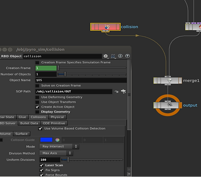
Let’s ignore outputs (2) and (3) for now. As you remember from Part 1 of the Tutorial, first we need to take care of the Pyro sim that will drive the overall shape of our cigarette smoke. But unlike in Part 1, we now have the dome as a collision object! So let’s go ahead and add this piece into the Pyro Sim.
To cache this sim make sure to keep things light and fast. Drop a GridMarkets Cache SOP and make sure to keep the path relative to $HIP; this way GridMarkets will have no problem re-creating a mirror of your local directory structure on their servers. On GridMarkets this sim took about 1 minute and 0.03$. Not bad at all!
This is roughly how your Pyro Sim should look like. Notice how thick the collision object is - this is to make sure the smoke doesn’t get out of the dome.
Note: I set my frame range to 1-240. In this tutorial I extended the frame range ‘cause I want to see some more of that sweet smoke accumulation under that dome!

Please note that I added an additional “Version” parameter to the GridMarkets OTL, ‘cause I want to control the path with a version number as well.
Now, assuming you have the same setup we built in the previous tutorial, we are ready for simulating the smoke lines. Let’s run the simulation and let’s focus for a moment on the very bottom, where the particles get emitted.
Everything seems ok-ish, but … if you visualize the lines (visualize the Add SOP connected after the Solver), something really doesn’t look right.
Why is this happening ?
The problem is most probably the following: In the Solver we are re-sampling the curves at a fixed step size (0.01 units). Now of course this operation would work wonders if the line we are about to re-sample were at least a little bit longer than 0.01. The problem is that at the very beginning of the simulation, the just-born points are still very very close to the emission point. So the lines that we create in this very early stage of the sim are too short to be resampled, collapsing into a null segment. Fortunately, after a few cycles, the points manage to go far enough to compensate this issue and the lines grow strong and healthy. But what about the first frames, the ones where we see the issue?
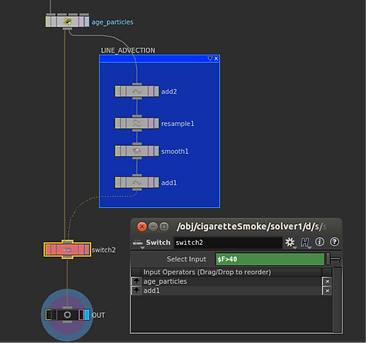
Well .. a very quick and relatively dirty solution would simply be to delay the following process (in Solver):
-
Create line
-
Resample
-
Smooth
-
Delete line
… say by 40 frames? Let’s give the points some time to grow into long
enough lines, with a very strategic Sw
Let's try again:
It seems to work reasonably well. We're now ready for rendering.
Here is the plan:
-
Create an Age point attribute.
-
Scatter a lot more lines to fill the gaps as best as we can.
-
Convert the lines into Volumes
-
Assign a Volumetric shader, add a Camera, a Light, a Mantra Rop and submit the render to the GridMarkets Cloud.
Why the Age step? Well, apart from the fact that I have a strong feeling that a bit later in this tutorial we’ll need it, in general, it’s always a good habit to have an attribute that helps to identify our lines’ (or particles in general) growth direction and progress.
Let's initialize a point attribute f@age outside the Solver SOP.

Use GridMarkets’ Cache SOP to cache this sim in a similar fashion as before.
… and let’s increase the particle age at every time step by the time step value. Note that the time step value is given by (Time) / (Frames per second).
In case we’re on a 24 fps setup, in VEX it would be @Time / 24.0. But (lucky us) there is a pre-built Vex attribute that returns this exact value : @TimeInc

Let's change the number of scattered points to 1000:

Now we can finally cache our Sim and the resulting lines!
I submitted this Sim to GridMarkets and it took about 1 hour to simulate and
It took 8 minutes to render and cost $3.6.
This is the resulting sim:

And here’s a close up:
As I’m sure you all have noticed with disappointment, our sim overtakes the dome in the upper part. Not good, not good at all!
But there is an easy fix. And once again VDB SDF is saving our invaluable time. Remember at the beginning of the tutorial when I wrote “Let’s ignore outputs (2) and (3) for now.”? Now it’s time to use output (2).
Let's import the SDF in cigaretteSmoke obj and use it to post-process the sim points using a Point Wrangle SOP.

Let’s analyze the code in the Point Wrangle for a moment: As we know SDF means “Signed Distance Field”. Meaning that every voxel of the SDF Volume contains the distance to the surface that originally generated it. How do we distinguish the voxels that are outside from the ones that are inside the surface? By the sign: The distance value will be positive if outside the original surface and negative if inside. So if we sample each sim point against the SDF, we do know for certain if the point is inside the dome or outside! This solves 50% of the problem.
The remaining 50% of the problem consists of moving the overtaking points back inside the dome. This is where the Gradient of the SDF field comes in handy. As I explained in Part 1 of my Tutorial, we can think of the gradient as the normal vector of a scalar field. In this case, of a SDF! So at this point we know the amount of space we need to push the points in, and even the direction (the gradient vector).
Reading the code in natural English, it would sound something like this:
For every point position P in the Sim:
-
Fetch the distance ‘dist’ from P to the dome surface
-
If the ‘dist’ is positive it means that the point is outside the dome. In this case:
-
Fetch the normal ‘grad’ on the surface from P
-
Move the point along ‘grad’ (the normal) by the amount ‘dist’. Just enough to stick the point on the dome surface.
-
And the problem is fixed. Thank you VDB !
Let’s render this thing!
I decided to render this fx as volumes. So we’ll need to find a way to convert those lines into a volume (VDB of course: It would be madness not to take advantage of sparse volumes for this fx, since we are sampling very thin lines).
In order to convert the lines into volumes we could initialize an empty VDB, activate it using the simulation bounding box and use a Volume Wrangle to sample each point into the VDB. All necessary steps of course… OR we can use a Volume Rasterize SOP, which performs all the steps above for us transparently!
Before doing that we need to set pscale and density for our points, ‘cause those will dictate the thickness and density of our Volumetric Smoke. Furthermore, in Volume Rasterize SOP set “Merge Method” to “Maximum”. “Add” will cause the density to accumulate where there are a lot of points, and I didn’t want that. But please feel free to experiment with this parameter.

By default, Volume Rasterize will just sample the points using their radius (pscale). We want to multiply that value by the density point attribute that we just created; this way, later we can modulate the density.
So, dive in the Volume Rasterize node and make sure to weigh the volume density with the actual point attribute “density”, as shown in the picture below.

Now visualize the Volume Rasterize node and this is roughly what you should see in your viewport.
Now let’s create a Material SOP, a ‘basicsmoke’ Mantra Shader, and make the proper shader assignments as shown below.


Don’t worry if this looks bad. Houdini OpenGL viewport has its limits and cannot visualize big volumes with a small voxel size. But fear not! This is just a visualization issue. Mantra will render every single voxel properly as we’ll see in a moment.
Note that in the Point Wrangle above I set density = 10.0, which is definitely too high for our render. The reason I set it to 10.0 is because it’s the only way to actually have some visual feedback in the viewport. So, now that we made sure everything works, feel free to set the density to 1.0 in the point wrangle, and from now on we’ll tweak the density only in the shader, ‘cause this will NOT require the Volume Rasterize to re-rasterize the volume at every density change.
It’s now time to add the remaining ingredients to this recipe: Camera, Area Light , Env Light and a Mantra ROP. Please feel free to position these elements according to your artistic sensitivity.
Looks promising! But there’s something I don’t like:
-
The base and tip of the smoke is too sharp (I want it to fade in)
-
The lines are too crisp (I can almost see each line)
How can we address all this? The overall problem is that the density is too high. We need to find a good balance.
Furthermore, and this is very important: Make sure to view your render on the actual shot plate. If the plate is not available yet (as it happens often) just download something from the Internet and slap comp your render on top of it. Why? Well, let’s try.
I’ve downloaded a random picture from Google Image and used it as environment map in my Env Light (Make sure to enable the checkbox “render light geometry” on the light parameters.) Now in my Mantra node I’m using both this Env Light and the Directional Light mentioned above.
As you can see, the look is very different! The sparse lines are now barely visible and the fact that the smoke doesn’t fade in in the lower part no longer bothers me that much.
BUT …
Let’s assume for a moment that your final render is on a very dark, maybe black, background and let’s take care of that “fading in” we wanted before my slap comp rant.
We want to remap age to a value between 0 and 1, corresponding to the beginning and end of every line. In order to do so, we need to find the current age at every frame. Which is the maximum age, so we can just use an Attribute Promote SOP set to “Maximum” and create a max_age detail attribute.
And I’ll go ahead and just render frame 120:


Now here’s the tricky part : In the Point Wrangle node that takes care of creating pscale and density, let’s create an additional float parameter “Fit Age Max” and let’s populate this parameter with the maximum age. This works great ‘cause every line has the same maximum age.
The expression seems more complicated than it is: opinputpath(“.”,0) returns a string containing the path of the node connected to this node (“.”) in the first input (0). And detail( …. , “max_age”, 0) returns the detail attribute we created in the previous step containing the maximum age for the whole sim.
In the body of the VEX code this is what’s going on:
For every point:
-
Get the maximum age of the whole smoke sim (fit_age_max).
-
Now that we know the age range, we can remap it to the range [0:1] with the VEX code fit(f@age, 0, fit_age_max, 0, 1), so we can feed this value into a ramp parameter (age_remap).
-
This is finally our density (f@density = … )
-
The point radius (pscale) is unchanged , and we assigned a color (Cd) as a visual feedback for the ramp we just created (red = low density, green = high density).
Now we can finally ‘draw’ our density creating a nice fade in and out using the Ramp, as shown below.


Now if we play the sim we should see this in the viewport (note this is not realtime. The first frames will be very fast, the last frames might take more than 20 second each to compute).
Just as expected : the tip of the smoke is red (meaning very low density, and the central part is green, high density).
Now we can finally submit a full render to GridMarkets! Please check the bottom part of this article for the stats about using GridMarkets for this project. This is the result:

Now let’s render the dome. Remember at the beginning of the tutorial when I wrote “Let’s ignore the outputs (2) and (3) for now.” Now it’s time to use output (3) !
At this point all we need to do is a quick comp. I won’t go into details about how to comp this, ‘cause compositing is a bit beyond the scope of this tutorial, but I attached a simple Nuke script below so you can have an idea of the main steps.
And here is the final result:
I hope you’ve enjoyed this article. Please feel free to download the hip file containing the whole setup and the nuke script. I have also included a handy environment map. Don’t hesitate to contact me if you have questions.
And as mentioned at the beginning of this article, don’t forget that you can find Part 1 of the Tutorial here : http://pepefx.blogspot.com/2016/04/cigarette-smoke.html
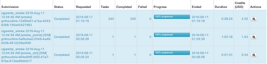
GridMarkets Simulation and Render Stats:
Using the GridMarkets Cloud Render Farm for this project was essential.
Sim + Render took about 1 hour and 20 minutes, and the total cost was about ~6$ for 240 Full HD frames. Not bad at all!
Alessandro Pepe 2016
By: Patricia Cornet
GridMarkets marketing